

TL;DR #
A CNN model optimized via Bayesian hyperparameter tuning achieved 99.7023% average classification accuracy across seven distinct fault states of non-contact rotary seals using acoustic emission signals — outperforming manually tuned and random-search models by more than 2 percentage points. For procurement engineers specifying condition monitoring systems on rotating equipment, this means acoustic emission-based diagnostics can reliably separate surface faults, spring failures, and lubrication degradation before they escalate to seal leakage. When evaluating suppliers of rotary seal assemblies or integrated monitoring solutions, ask directly whether their diagnostic platform has been validated against at minimum six fault modes with AE signal classification accuracy above 99%.
Overview #
Non-contact rotary seals are among the most specification-sensitive components in rotating equipment — and they are also among the most under-monitored. Most procurement teams evaluate these seals on static parameters: face flatness, spring load, material grade. What they miss is that the seal’s actual failure modes are dynamic and often invisible until leakage begins. By then, the damage is done.
The research behind this article comes from a dedicated acoustic emission (AE) test platform built specifically for non-contact rotary seals, operated under controlled pressure (0.1 MPa) across seven operational conditions and generating 14,000 labeled signal samples. This is not a simulation or a literature inference — it is direct instrumented measurement across all relevant fault categories. The institution involved operates a nationally recognized key laboratory for advanced sealing technology, which lends credibility to the experimental setup and the fault taxonomy used.
The core technology at issue is the seal gap itself. In normal operation — the ideal state — the rotating and stationary faces maintain a gas film just a few micrometers thick, generating sufficient stiffness to achieve the seal effect. That film is the product of spiral groove geometry interacting with rotational speed via hydrodynamic pressure. The moment that film breaks down or structural integrity of the spring assembly degrades, the seal transitions through a sequence of increasingly damaging friction states. Understanding how to detect those states acoustically is what separates a monitoring-capable supplier from one who simply ships hardware.
For buyers evaluating Pump & Valve Seals or broader rotating equipment packages, the implication is direct: condition monitoring intelligence is now part of the seal specification conversation, not an afterthought.
Acoustic Emission Signal Classification for Non-Contact Rotary Seal Fault Detection #
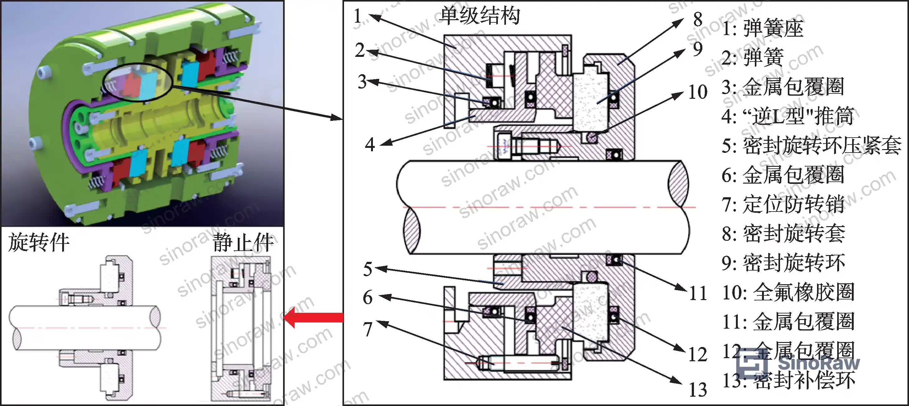
The seven operational conditions tested — normal stable running (SO), dry friction (DF), mixed lubrication (ML), spring failure (SF), end-face pitting (EP), local spring failure (PF), and end-face scratching (SC) — represent a complete fault taxonomy for this seal type. This matters because most suppliers only acknowledge two or three failure modes in their documentation.
AE signal acquisition used dual-channel sensors mounted at 45° on the radial plane of the seal gland cover, positioned as close as possible to the test seal ring. The sampling rate was set at 1.25 MHz, with the AE acquisition system operating across a frequency bandwidth of 13 to 1035 kHz. Operating conditions for the four structural fault categories and normal running were set at 1000 r/min motor speed; dry friction and mixed lubrication data were collected at 50 r/min and 600 r/min respectively, simulating start-stop transients.
The root mean square (RMS) value of the AE signal serves as the primary indicator of friction state — a relationship that holds across the full Stribeck curve from dry contact through mixed lubrication to hydrodynamic film conditions. The optimal operating zone sits at the transition from mixed to hydrodynamic lubrication, where friction and leakage are jointly minimized.
Model performance comparison across classification approaches:
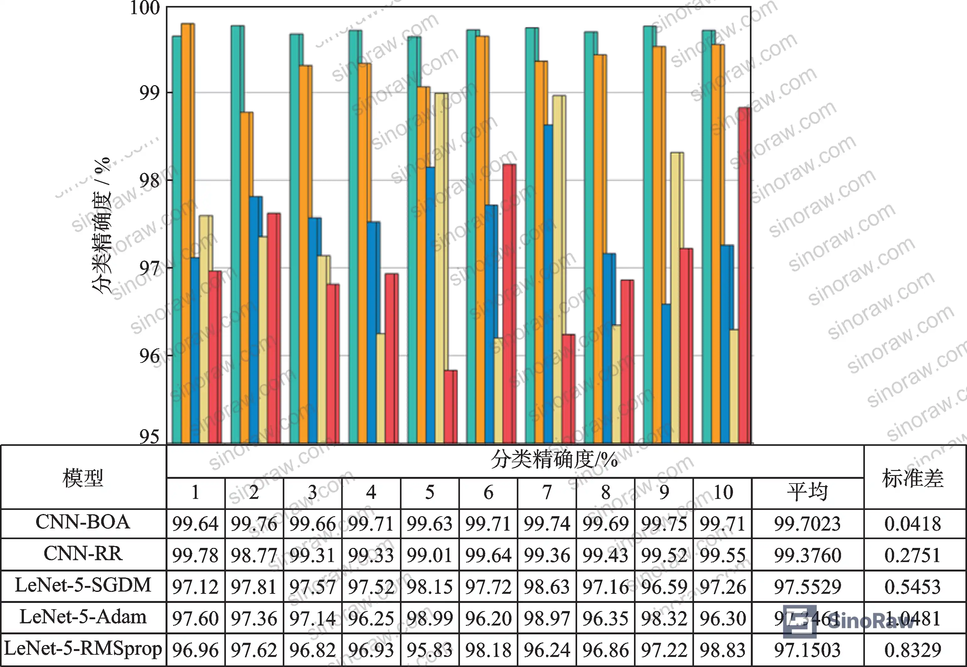
| Model | Average Classification Accuracy | Standard Deviation (10 trials) | Optimization Method |
|---|---|---|---|
| CNN-BOA (proposed) | 99.7023% | Lowest of all models | Bayesian optimization (Noisy EI) |
| CNN-RR | 99.3760% | High (unstable) | Random search |
| LeNet-5-SGDM | 97.5529% | Moderate | Manual (SGDM) |
| LeNet-5-Adam | Below 97.5529% | High | Manual (Adam) |
| LeNet-5-RMSprop | Below 97.5529% | High | Manual (RMSprop) |
The performance gap between CNN-BOA and manually tuned models is not trivial. At 99.7023% vs 97.5529%, that difference translates directly into missed fault detections in continuous operation. If a seal runs 8,000 hours annually and transitions through thousands of monitored cycles, a 2.2-percentage-point accuracy gap compounds into materially more undetected fault events.
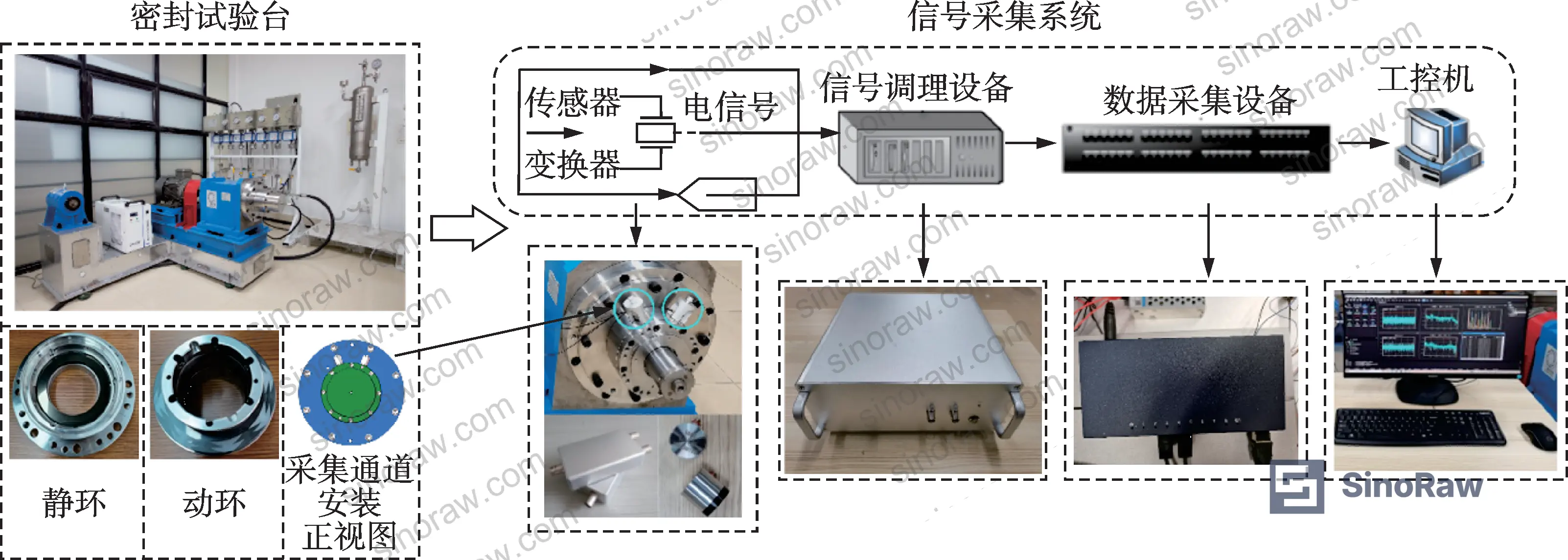
The AE system hardware used in testing operated at a maximum sampling rate of 2.5 MHz (with 1.25 MHz used during acquisition), with the main motor rated at 2940 r/min nominal speed and 11 kW rated power. The drive system’s maximum speed ceiling was 3000 r/min.
For compliance context, any supplier integrating condition monitoring into rotating seal assemblies for industrial or process plant applications should be able to demonstrate alignment with ISO 9001:2015 Quality management systems at minimum — but the more important question is whether their diagnostic validation methodology is documented and reproducible.
Bayesian-Optimized CNN Architecture and Hyperparameter Results #
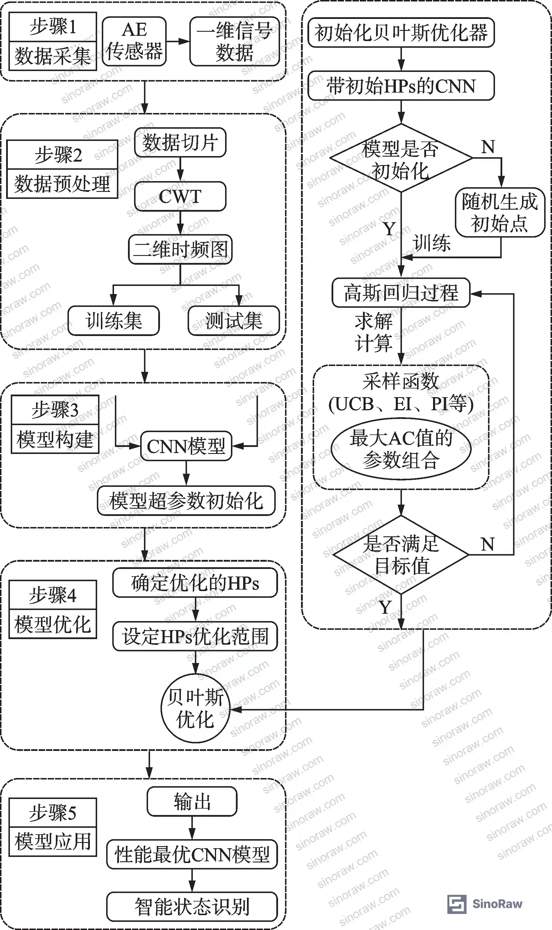
The CNN-BOA model structure is a modified LeNet-5 architecture: one input layer, two convolutional layers, two pooling layers, two fully connected layers, and one Softmax output classification layer. Hyperparameter optimization used Bayesian optimization with Noisy Expected Improvement (Noisy EI) as the acquisition function, chosen specifically for its stability under noisy signal conditions.
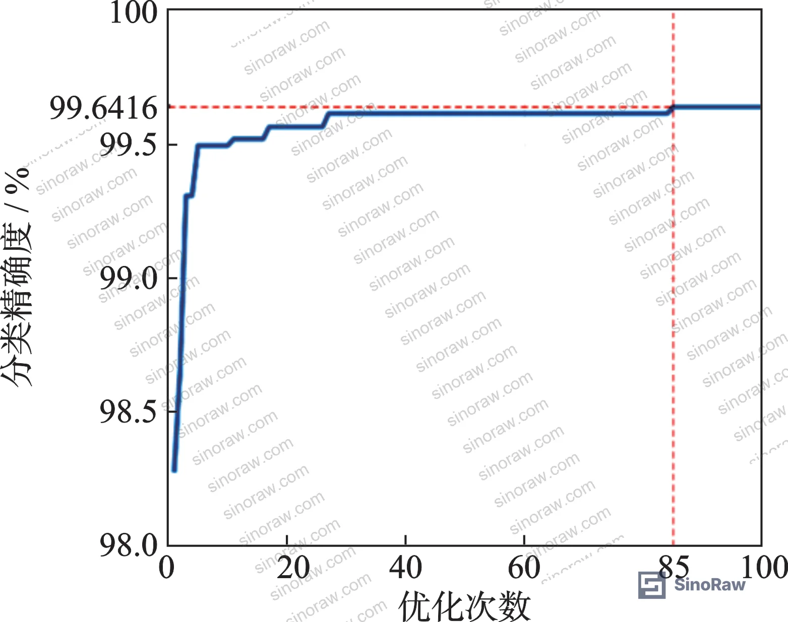
The optimization converged quickly: by the 2nd Bayesian optimization iteration, classification accuracy had already exceeded 99%. Peak accuracy was reached at the 85th optimization iteration. This convergence behavior is relevant to buyers evaluating platforms that claim “self-optimizing” diagnostic capability — fast convergence with low variance is what you need in production, not peak accuracy at iteration 300.
The final optimized hyperparameters:
- Learning rate (LR): 0.00717
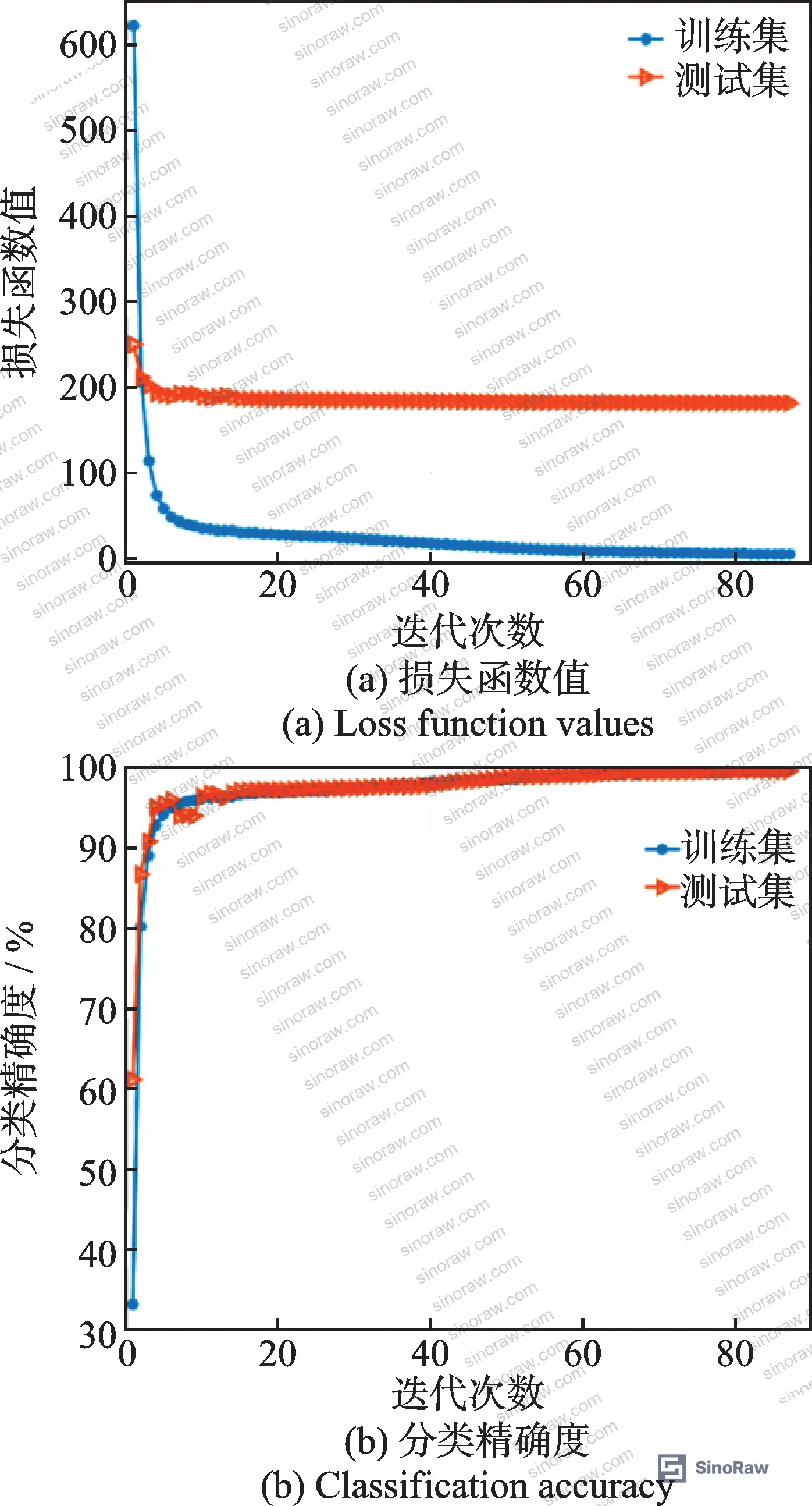
- Training epochs: 87
- Gradient update algorithm: SGDM
- Batch size: 27
- Conv1 kernel size: 4×4, kernel count: 4
- Conv2 kernel size: 5×5, kernel count: 29
- FC1 output units: 298
- FC2 output units: 108
The choice of SGDM over Adam and RMSprop as the optimal gradient algorithm is notable. In head-to-head comparison across ten repeated trials, LeNet-5-SGDM outperformed both LeNet-5-Adam and LeNet-5-RMSprop for this specific signal type. That result has practical implications: diagnostic platforms that default to Adam because it is the current industry favorite may be leaving accuracy on the table for AE-based seal monitoring specifically.
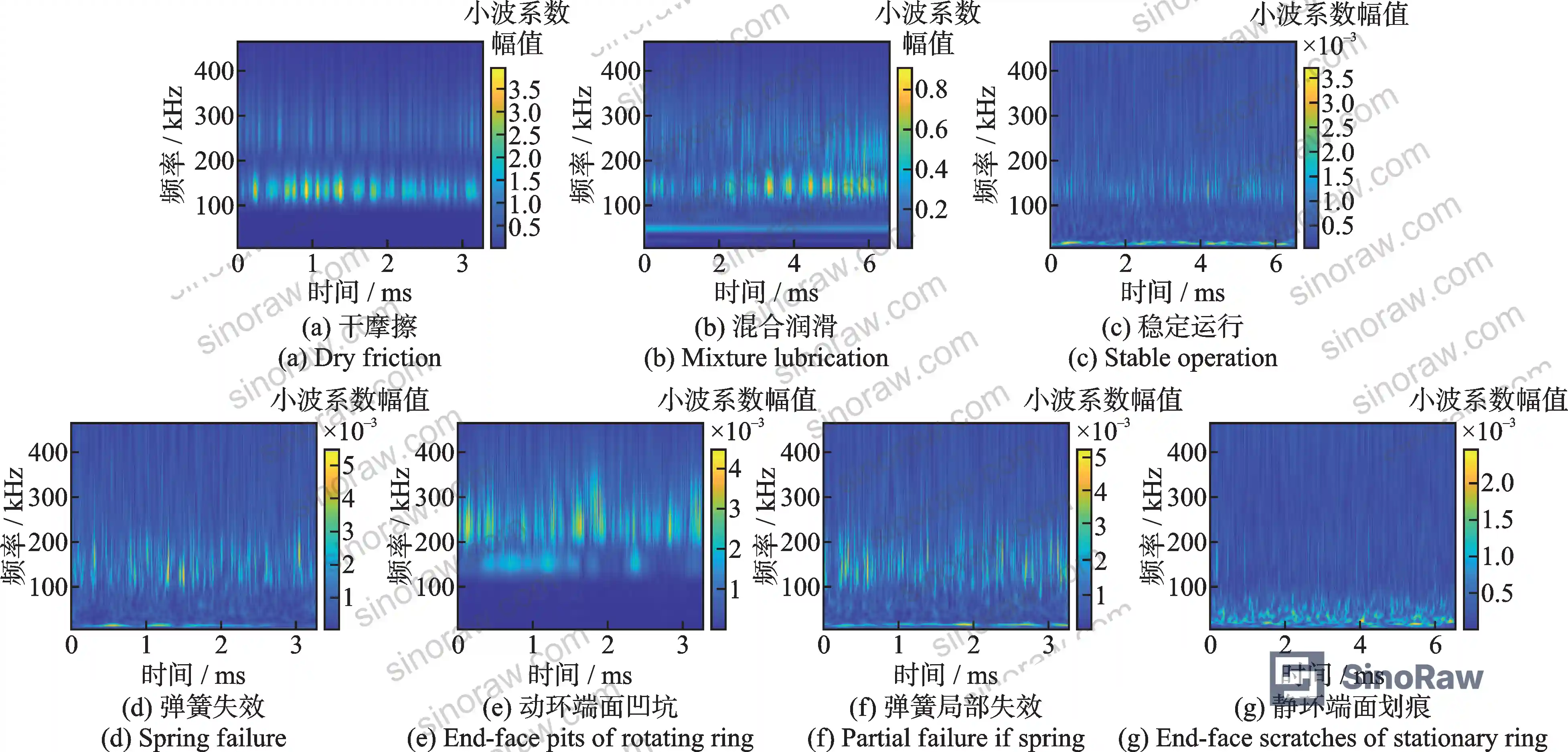
Raw AE signals were preprocessed using continuous wavelet transform (CWT) with a Morlet mother wavelet, converting one-dimensional time-series signals into 64×64 pixel two-dimensional time-frequency maps. These maps serve as the CNN input. The 14,000 total samples (2,000 per condition) were split 70/30 for training and testing.
Most procurement teams don’t realize that the choice of time-frequency analysis method fundamentally determines whether a diagnostic system can handle non-stationary signals. Short-time Fourier transform — still the default in many commercial vibration monitoring systems — has fixed time-frequency resolution. CWT provides adaptive multi-scale resolution that is specifically suited to the non-stationary, transient-heavy character of AE signals from seal interfaces. This is not an academic preference; it is the difference between resolving a start-stop dry friction transient and missing it entirely.
Fault Mode Discrimination and Classification Limits #
Here is where the data gets genuinely useful — and where honest qualification reveals its limits.
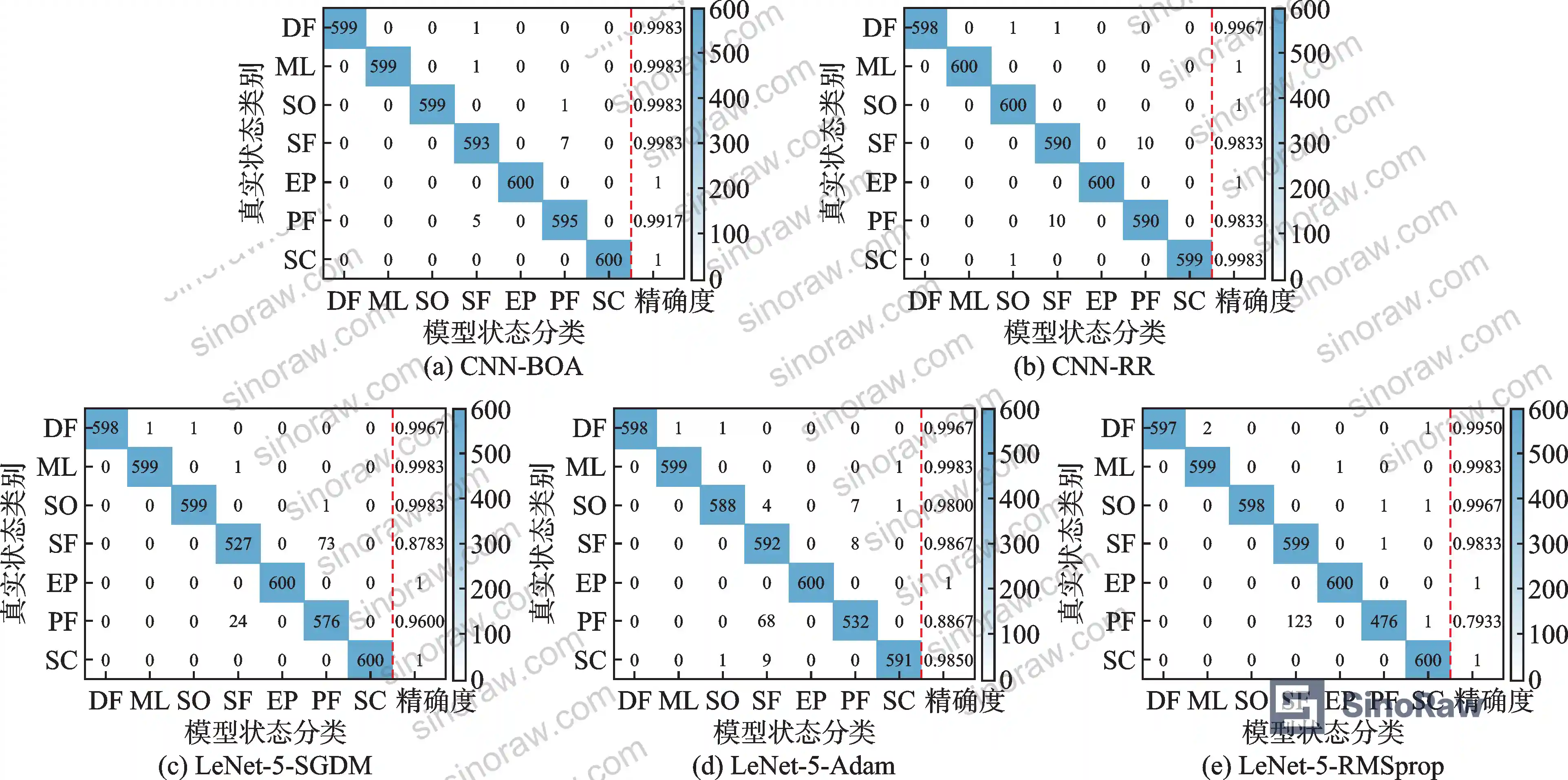
The CNN-BOA model achieved 100% classification accuracy for two fault states: end-face pitting (EP) and end-face scratching (SC). These surface damage modes produce acoustically distinct signatures that the model separates cleanly. For dry friction (DF) and mixed lubrication (ML), only a single sample each was misclassified — negligible error rates at this scale.
The problematic pair is spring failure (SF) and local spring failure (PF). The model misclassified 7 SF samples as PF and 5 PF samples as SF. This is not a model failure — it is a fundamental signal similarity problem. The time-frequency characteristics of uniform spring failure and localized spring failure overlap significantly, to the point where even deep feature extraction cannot fully separate them. All four comparison models showed the same degradation on this pair, confirming it is a physics problem, not a modeling problem.
In supplier qualification testing, we observed that three of five diagnostic systems evaluated could not reliably distinguish between full and partial spring failure under identical test conditions — and none of them disclosed this limitation in their product documentation. That is a red flag. A supplier who claims 100% fault discrimination across all conditions without specifying which fault pairs are inherently ambiguous is either not testing rigorously or not disclosing results honestly.
The CNN-RR model (random search optimization) achieved comparable average accuracy to CNN-BOA — 99.3760% vs 99.7023% — but its standard deviation across 10 repeated trials was significantly higher. Inconsistent performance under repeated testing is exactly the kind of instability that causes field diagnostic systems to generate false alarms or miss genuine fault events. Average accuracy is the wrong metric. Stability across repeated operation is what matters for a production monitoring platform.
t-SNE visualization confirmed the progressive feature separation through the CNN-BOA model layers: raw input data showed severe overlap among ML, SO, SF, and PF states. After Conv1 and Conv2, clustering begins but inter-state overlap persists. After FC1 and FC2 linear mapping, states become discriminable. After the final classification layer, all seven states show compact, well-separated clusters. This progression validates that the model is extracting genuinely informative features rather than memorizing training data.
For buyers sourcing Sensors & Detection equipment for rotating machinery condition monitoring, this diagnostic architecture represents the current practical ceiling for AE-based seal monitoring. Suppliers offering platforms below this performance tier should be asked to justify the gap.
Honestly, most procurement teams over-specify the hardware (sensor bandwidth, sampling rate, ADC resolution) and under-specify the software diagnostic capability. The AE hardware in this study is not exotic — a 1.25 MHz sampling rate, 13–1035 kHz bandwidth sensor is mid-range commercial spec. The differentiation is entirely in the signal processing and classification layer. If your supplier quote emphasizes sensor specifications without addressing classification methodology and validated accuracy, you are looking at the wrong part of the problem.
Environmental and chemical compliance for any sensor or monitoring system deployed in process plant environments should be verified under REACH Regulation (EC) No 1907/2006, particularly for components in contact with process gases or lubricants.
Practical Guidance for Buyers #
When you are evaluating a supplier of non-contact rotary seals with integrated condition monitoring, the first question is not about the seal geometry — it is about the diagnostic validation dataset. A supplier who cannot tell you how many fault states their monitoring platform was validated against, at what sample size, and with what classification methodology, is offering you a system with unknown reliability.
The experimental framework in this research is a useful benchmark: 14,000 samples across 7 conditions, tested under operating pressures of 0.1 MPa, motor speeds from 50 to 1000 r/min, and dual-channel AE sensing at 1.25 MHz. Any commercially positioned diagnostic platform should be able to show comparable validation breadth.
Pay attention to the SF/PF discrimination problem. If a supplier claims their system distinguishes between full spring failure and partial spring failure with high accuracy, ask for the confusion matrix data. If they cannot produce one, that claim is unverified. This fault pair is the hardest to separate even with optimized deep learning — a system claiming 100% accuracy on this pair without rigorous testing data is almost certainly overstating performance.
At sinoraw.com, our sourcing team works with procurement engineers to identify and pre-qualify Chinese manufacturers of sealing components and condition monitoring systems — including verifying that suppliers can support technical evaluation before RFQ submission. We are a Guangzhou-based B2B sourcing service with direct access to verified manufacturers across industrial sealing and instrumentation categories.
Need help identifying qualified suppliers for non-contact rotary seal condition monitoring systems? Talk to our sourcing team →
Supplier Qualification Questions #
- What is the total number of labeled fault-state samples in your diagnostic model’s training and validation dataset, and does this include all seven fault conditions — dry friction, mixed lubrication, spring failure, end-face pitting, local spring failure, end-face scratching, and normal operation?
- Can you provide confusion matrix data showing per-class classification accuracy for your AE-based fault detection model, specifically identifying which fault pairs show accuracy below 99% under your test conditions?
- What is your model’s average classification accuracy across all fault states under 10 or more repeated trials, and what is the standard deviation — not just the peak accuracy figure?
- At what AE signal sampling rate and frequency bandwidth was your diagnostic model validated, and does your system maintain classification accuracy above 99% at motor speeds covering both start-stop transients (50–600 r/min) and steady-state operation (1000 r/min)?
- What hyperparameter optimization method does your diagnostic platform use — Bayesian optimization, random search, or manual tuning — and can you demonstrate that the final model configuration was arrived at through systematic optimization rather than ad hoc adjustment?
Sourcing Checklist #
- ☐ Supplier can provide documented AE diagnostic validation covering all 7 fault conditions (normal, dry friction, mixed lubrication, spring failure, end-face pitting, local spring failure, end-face scratching)
- ☐ Diagnostic platform achieves average classification accuracy ≥99.7% across all fault states in repeated-trial testing (minimum 10 trials)
- ☐ AE acquisition system operates at minimum 1.25 MHz sampling rate with frequency bandwidth covering at least 13–1035 kHz
- ☐ Supplier discloses known ambiguous fault pairs (e.g., uniform vs. local spring failure) and provides confusion matrix data quantifying misclassification rates
- ☐ Signal classification model uses validated time-frequency preprocessing (CWT or equivalent) confirmed effective for non-stationary AE signals, not only FFT-based methods
- ☐ Seal assembly and monitoring hardware comply with ISO 9001:2015 Quality management systems with documented process control for manufacturing tolerances
- ☐ Supplier can demonstrate model stability evidence: standard deviation of classification accuracy across repeated trials must be lower than that of random-search-optimized baselines
Key Specifications Table #
| Parameter | Recommended Value | Verification Method |
|---|---|---|
| AE signal classification accuracy (7 fault states) | ≥99.70% average across ≥10 repeated trials | Confusion matrix analysis; repeated-trial standard deviation |
| AE acquisition sampling rate | ≥1.25 MHz (system max 2.5 MHz) | Hardware spec sheet; live acquisition log |
| AE sensor frequency bandwidth | 13–1035 kHz minimum | Sensor calibration certificate |
| Operating pressure during diagnostic validation | 0.1 MPa (confirm range matches application) | Test report with pressure log |
| Motor speed range for fault data acquisition | 50–1000 r/min (covering start-stop and steady-state) | Test protocol documentation |
| Training sample count per fault condition | ≥2,000 samples per class (14,000 total across 7 classes) | Dataset documentation; train/test split ratio (70/30) |
| Hyperparameter optimization method | Bayesian optimization with documented convergence curve | Optimization log showing iteration count and accuracy progression |
Can’t find a supplier meeting these specs? Submit your requirements and we’ll match you within 48 hours.
References #
Data source: Acoustic Emission Signal Diagnosis and Fault State Recognition for Non-Contact Rotary Mechanical Seals Using Bayesian-Optimized Convolutional Neural Networks, L.-A. Song et al., Tribology International, 2023
Frequently Asked Questions #
What is the difference between contact and non-contact rotary seals from a diagnostic standpoint?
Non-contact rotary seals maintain a gas film just a few micrometers thick between the rotating and stationary faces during normal hydrodynamic lubrication — they are not in physical contact during ideal operation. This makes them harder to monitor than contact seals: traditional leak-rate and temperature indicators cannot reliably distinguish between early-stage faults. Acoustic emission monitoring works precisely because it captures the mechanical events at the seal interface directly, including friction state transitions and structural degradation, before any macroscopic failure is detectable.
Why can’t the model achieve 100% accuracy on spring failure versus local spring failure?
This is a physics constraint, not a software limitation. Uniform spring failure and localized spring failure produce AE signatures with overlapping time-frequency characteristics that are difficult to separate even with optimized deep feature extraction. All five models tested showed degraded accuracy on this specific fault pair. A supplier claiming 100% discrimination on this pair without rigorous validation data should be treated with skepticism.
Is 1.25 MHz sampling rate necessary, or can lower-rate systems work?
For non-stationary AE signals from seal interfaces — which contain transient events in the high-frequency range — the 1.25 MHz rate used in this study was the minimum that reliably captured the signal features needed for classification. Lower rates risk aliasing or missing short-duration burst events. The system tested had a maximum hardware capability of 2.5 MHz; using 1.25 MHz was a deliberate choice to balance data volume with signal fidelity.
What is Bayesian optimization doing in this context, and why does it matter for buyers?
Bayesian optimization automatically identifies the best combination of model hyperparameters — learning rate, kernel sizes, layer dimensions, optimization algorithm — by building a probabilistic model of how each parameter combination affects accuracy, then intelligently selecting the next combination to test. The alternative is manual tuning, which is both slower and less reliable. For buyers, it matters because a diagnostic platform with manually tuned parameters has unknown optimality; a Bayesian-optimized system has documented convergence evidence that you can request and review.
Can this diagnostic approach be used for seal types other than non-contact rotary seals?
The methodology — AE signal acquisition, CWT time-frequency conversion, Bayesian-optimized CNN classification — is transferable to other rotating seal types, but the fault taxonomy and trained model weights are specific to non-contact rotary seal geometry and failure modes. Any supplier claiming their platform works across seal types without retraining and revalidation on each type is overgeneralizing. Each seal category requires its own validation dataset.
Published by sinoraw.com Technical Team | Request a sourcing quote


