

TL;DR #
A deep learning model combining continuous wavelet transform with Bayesian-optimized CNN achieved 99.7023% average classification accuracy across seven distinct non-contact rotary seal fault conditions — including spring failure, end-face pitting, and dry friction — using 14,000 acoustic emission feature samples. For procurement engineers specifying condition monitoring systems for rotating seal applications, this data sets a concrete benchmark: any AI-based seal diagnostic platform claiming less than 99% classification accuracy under non-stationary signal conditions should be treated with skepticism. Before issuing an RFQ for seal monitoring equipment, require suppliers to demonstrate confusion matrix results across at least six fault categories under real operating pressure conditions.
Overview #
When a non-contact rotary seal fails in service, the traditional diagnostic approach — watching for leakage rates, temperature rise, or pressure drop — gives you information about the failure after it has already progressed to a critical stage. That is too late for predictive maintenance, and it forces procurement teams to over-specify safety margins across the entire seal selection. Recent research from a university-based advanced sealing laboratory in eastern China challenges this paradigm directly, using acoustic emission (AE) signal monitoring paired with an adaptive convolutional neural network to catch failure modes while they are still developing.
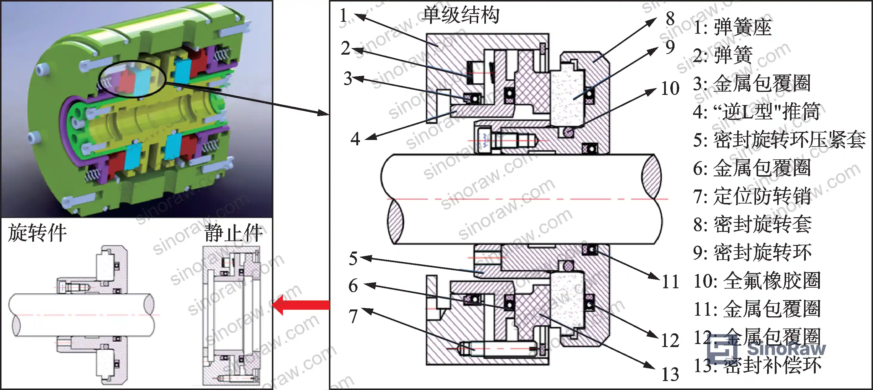
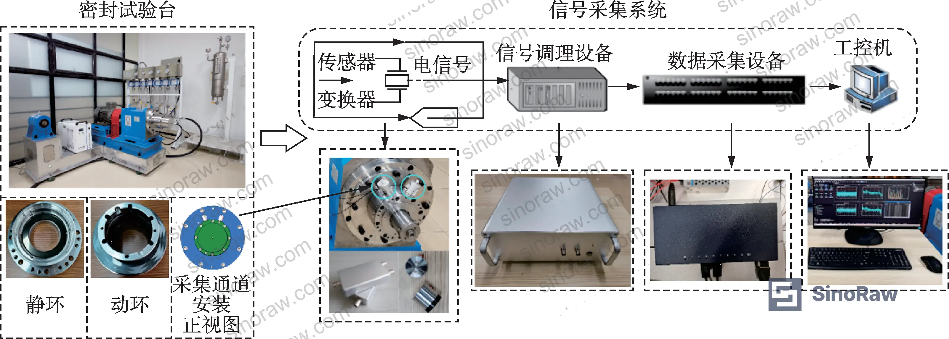
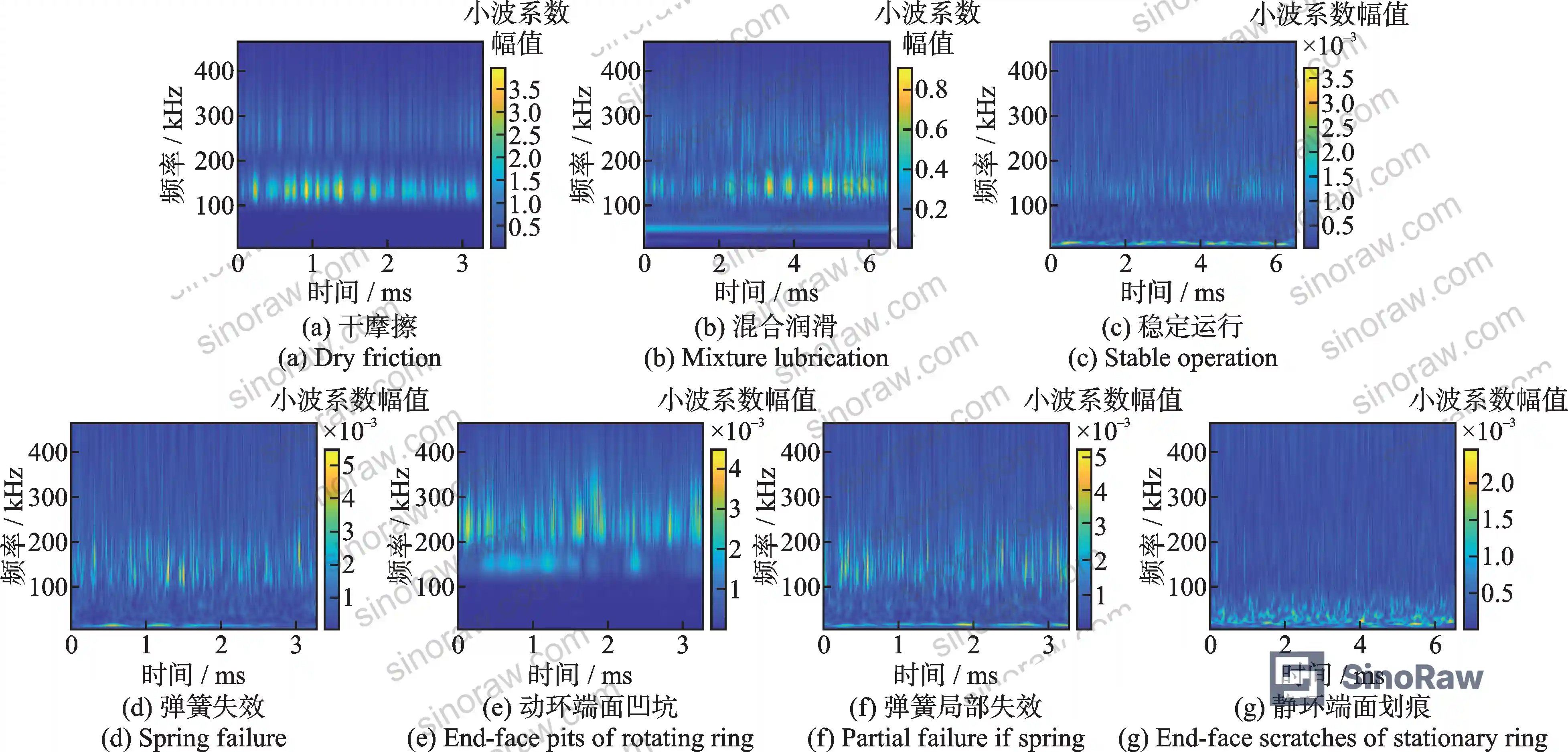
The experimental program covered seven operational conditions — normal running, dry friction, mixed lubrication, spring failure, end-face pitting, partial spring failure, and end-face scratching — generating a validated dataset of 14,000 feature samples collected at a sampling rate of 1.25 MHz across a frequency bandwidth of 13 to 1035 kHz. All tests were conducted at 0.1 MPa pressure. This is not a simulation study; the team built a dedicated test rig with a variable frequency drive controlling motor speeds from 50 r/min up to 1000 r/min to replicate the full range of tribological states a non-contact seal experiences from startup through steady operation.
For buyers sourcing condition monitoring solutions or evaluating seal diagnostic systems, this research provides one of the most precisely quantified fault classification benchmarks available for this component category. The implications for Pump & Valve Seals specification and Sensors & Detection equipment sourcing are direct and significant.
Non-Contact Rotary Seal Fault Classification: What the Data Actually Shows #
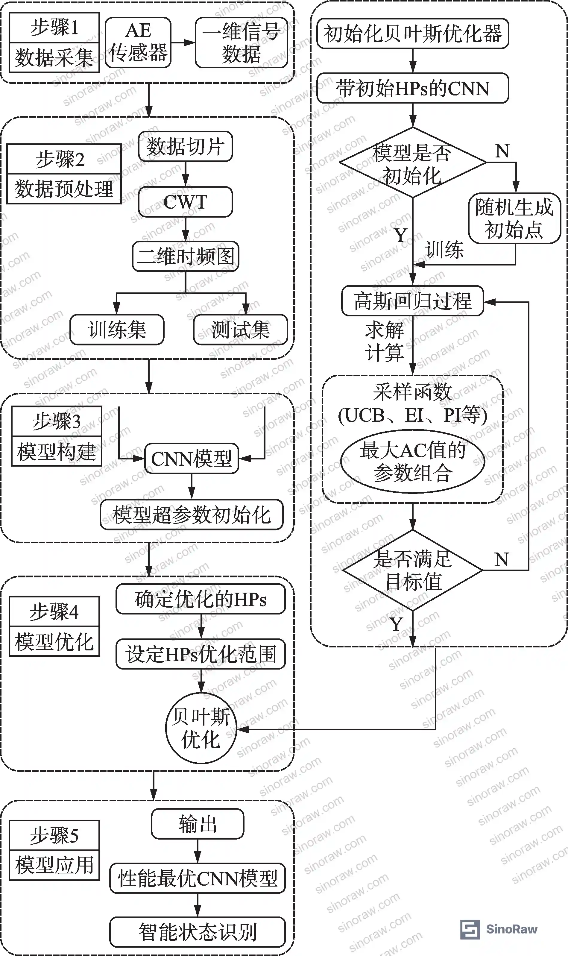
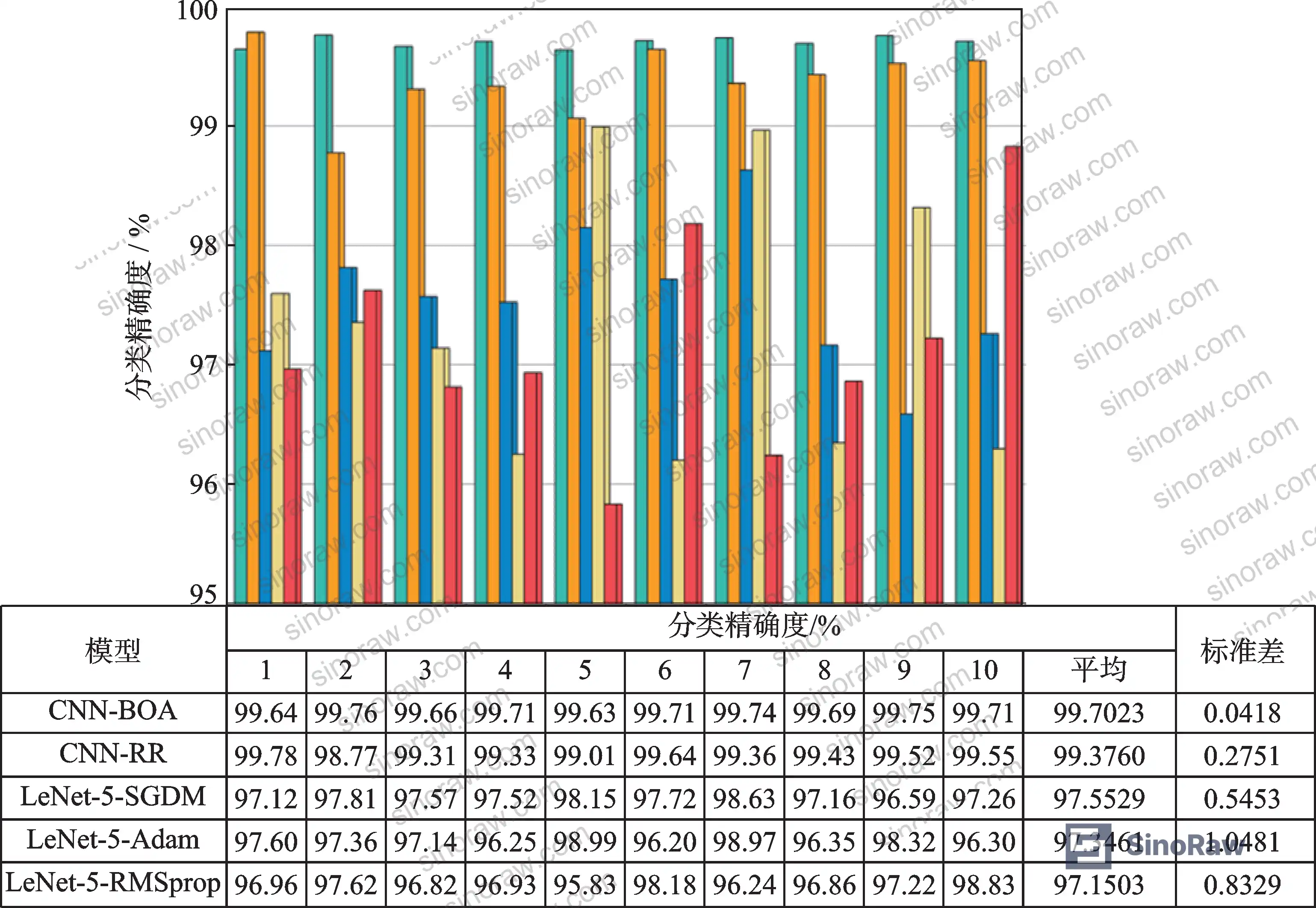
This is where the numbers get interesting. The CNN-BOA model — that is, the CNN architecture with Bayesian-optimized hyperparameters — achieved a mean classification accuracy of 99.7023% across all seven operating states. For context, the same architecture using random search hyperparameter optimization (CNN-RR) reached 99.3760%, and manually tuned LeNet-5 variants came in at 97.5529% on average. The difference between 97.5% and 99.7% sounds small until you calculate what it means across thousands of seal monitoring cycles in a continuous process plant.
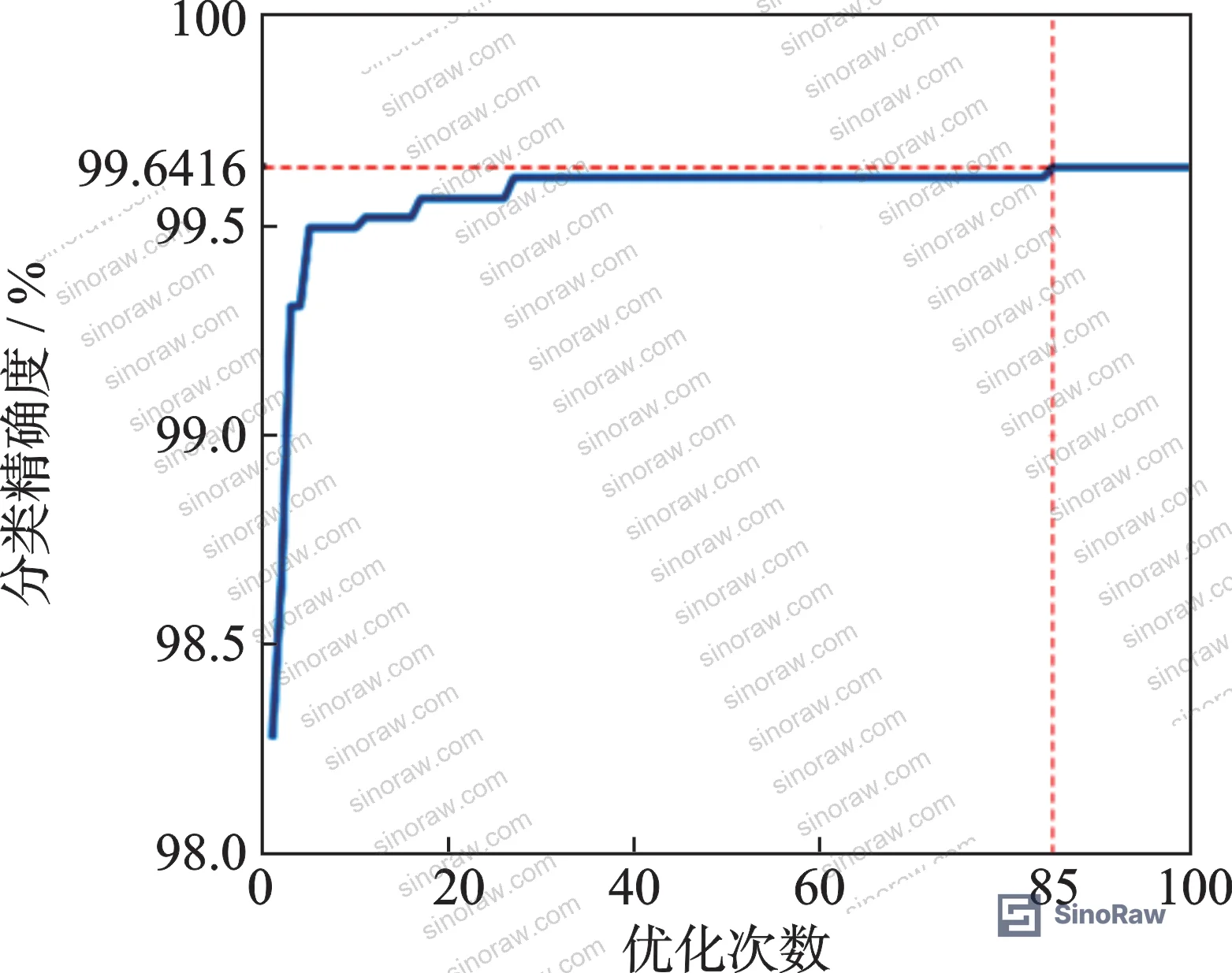
The Bayesian optimization converged meaningfully fast: by the second optimization iteration, classification accuracy had already exceeded 99%. The final optimized model used a learning rate of 0.00717, 87 training epochs, SGDM gradient optimization, and a batch size of 27. The two convolutional layers used kernel sizes of 4×4 and 5×5 respectively, with 4 and 29 output channels. Fully connected layers mapped through 298 and 108 intermediate features before the 7-class output layer.
Where the model struggled — and what that tells you #
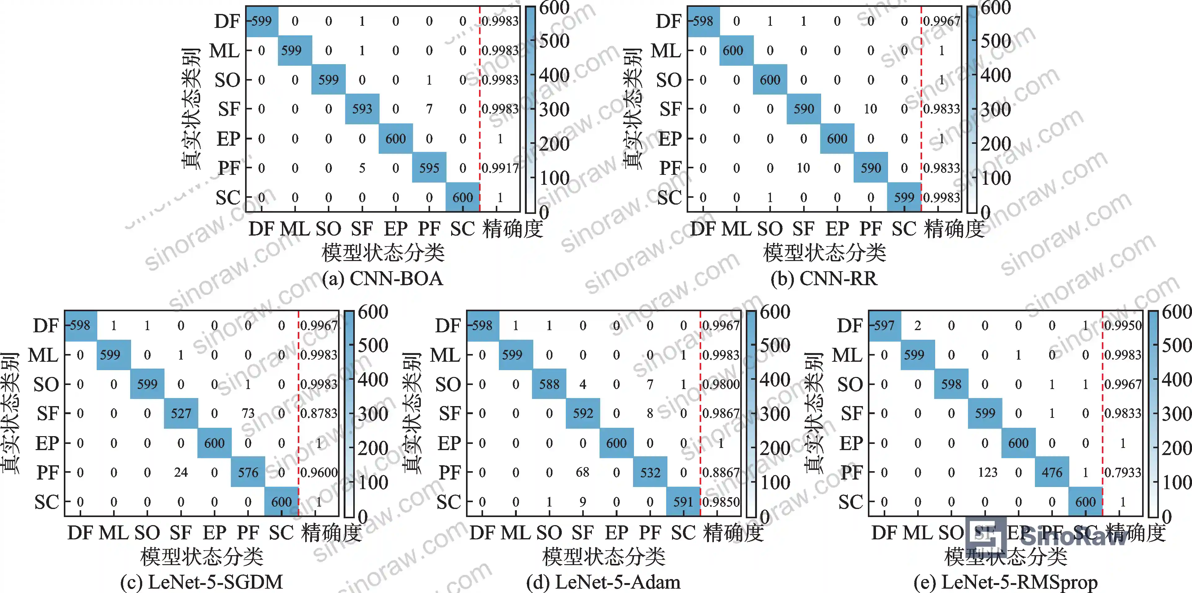
Honestly, most buyers assume that if a model hits 99%+ average accuracy, every fault class is equally well-separated. That is not what the data shows. End-face pitting (EP) and end-face scratching (SC) achieved 100% classification accuracy. Dry friction (DF) and mixed lubrication (ML) each had only a single sample misclassified — as spring failure (SF). But spring failure (SF) and partial spring failure (PF) showed meaningful cross-contamination: 7 SF samples were misclassified as PF, and 5 PF samples were misclassified as SF. This is a failure/friction point worth noting for buyers specifying seal monitoring systems.
The reason is physically intuitive: SF and PF share similar time-frequency signatures because partial spring failure is an intermediate degradation state of full spring failure. Even after full CNN feature extraction, the boundary between these two states is not perfectly clean. Any supplier claiming 100% classification accuracy across SF and PF in a real installation should be asked to produce their confusion matrix data.
Model comparison table #
| Model | Mean Classification Accuracy | Optimization Method | Stability (Std Dev) |
|---|---|---|---|
| CNN-BOA | 99.7023% | Bayesian optimization | Lowest (most stable) |
| CNN-RR | 99.3760% | Random search | Moderate (random sampling) |
| LeNet-5-SGDM | Best among manual-tuned group | Manual (SGDM) | Poor |
| LeNet-5-Adam | Lower than CNN-RR | Manual (Adam) | Poor |
| LeNet-5-RMSprop | Lowest | Manual (RMSprop) | Poorest |
The CNN-RR model’s average accuracy exceeded 99% but carried a substantially larger standard deviation than CNN-BOA across 10 repeated trials. That variance matters in production monitoring environments: you need consistent classification, not a model that occasionally spikes to 99.8% but routinely drops to 98.5%.
Acoustic Emission Signal Processing for Seal Fault Identification #
The signal processing pipeline is worth understanding in detail because it determines what hardware specifications actually matter when sourcing AE-based diagnostic equipment.
Raw one-dimensional AE signals were sliced and converted to two-dimensional time-frequency maps using continuous wavelet transform (CWT) with a Morlet mother wavelet. The resulting time-frequency images were 64×64 pixels per sample. This transformation is what makes CNN-based classification tractable: the CNN processes the image representation of the signal, not the raw waveform. The practical implication is that the sampling rate of the AE acquisition hardware is a hard constraint — the 1.25 MHz sampling rate used here, within a sensor bandwidth of 13 to 1035 kHz, is necessary to capture the high-frequency content that distinguishes these fault modes.
Most procurement teams don’t realize that the bandwidth specification of the AE sensor is often more critical than the sensor sensitivity rating. A sensor with a narrow bandwidth — say, 100 to 400 kHz — will miss the frequency components that separate dry friction from mixed lubrication states. The research used a system capable of 2.5 MHz maximum sampling rate with 13 to 1035 kHz bandwidth, which should be treated as a minimum capability benchmark for any AE-based seal monitoring system.
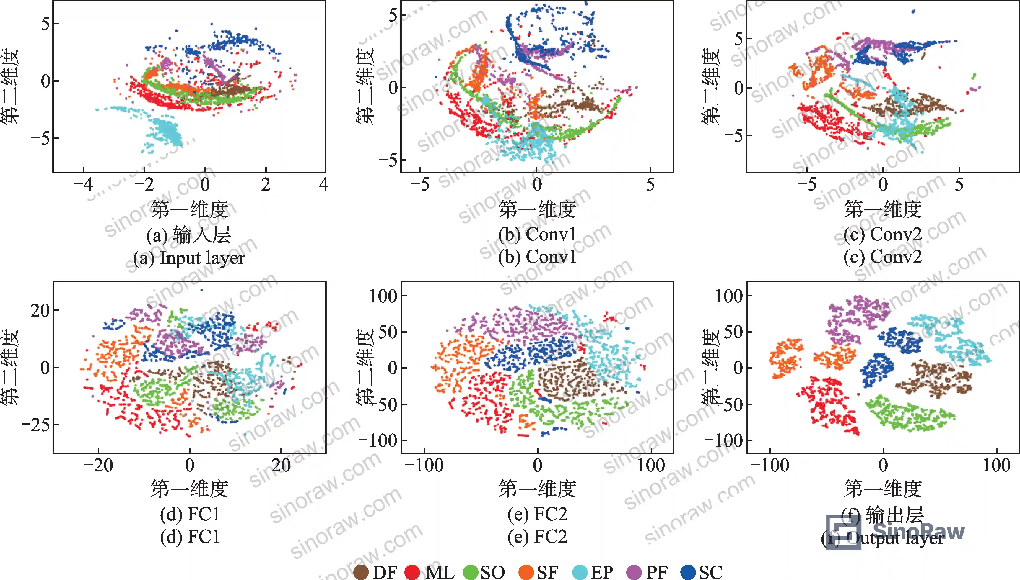
The t-SNE visualization results confirm what the confusion matrix data implies. Raw input data shows severe overlap between mixed lubrication (ML), normal operation (SO), spring failure (SF), and partial spring failure (PF) states in 2D feature space — these four states are essentially indistinguishable from raw signal data. After passing through both convolutional layers, same-state data begins clustering but remains partially overlapping. Only after both fully connected layers does the inter-class separation become reliable, and only after the classification layer are all seven states cleanly separated.
This progression matters for buyers evaluating whether an AE monitoring system’s edge processing hardware is sufficient. If the system is designed to make classification decisions before FC layers are computed — a common cost-cutting approach in embedded systems — you will see degraded performance on exactly the fault classes that matter most clinically.
Compliance requirements for industrial condition monitoring equipment typically intersect with ISO 9001:2015 Quality management systems certification for the manufacturer, but that alone tells you nothing about algorithm performance. Demand test data. Separately, if the monitoring system is deployed in chemical or petrochemical environments, check that sensor materials and housings comply with REACH Regulation (EC) No 1907/2006 on restricted substances — AE sensors with piezoelectric elements can contain regulated compounds.
Hyperparameter Optimization and Diagnostic Reliability #
The Bayesian optimization framework used here is directly relevant to any buyer evaluating AI-based predictive maintenance platforms — not just seal diagnostic systems. The key insight is that manually tuned models (LeNet-5 variants with SGDM, Adam, or RMSprop) showed high variance across repeated trials. The CNN-RR model also showed meaningful variance despite using automated search, because random search samples hyperparameter space without learning from previous evaluations.
The Bayesian approach — using a Gaussian process surrogate model updated iteratively via a Noisy Expected Improvement acquisition function — reduced hyperparameter search to 85 iterations to achieve peak performance. The final parameters: learning rate 0.00717, 87 epochs, batch size 27, Conv1 kernel 4×4 with 4 channels, Conv2 kernel 5×5 with 29 channels. These are not arbitrary numbers — they represent the output of a systematic optimization over 9 hyperparameter dimensions simultaneously.
For procurement purposes, this translates to a simple question: can the supplier show you the hyperparameter optimization history for their diagnostic model, or did they set those values manually and call it done?
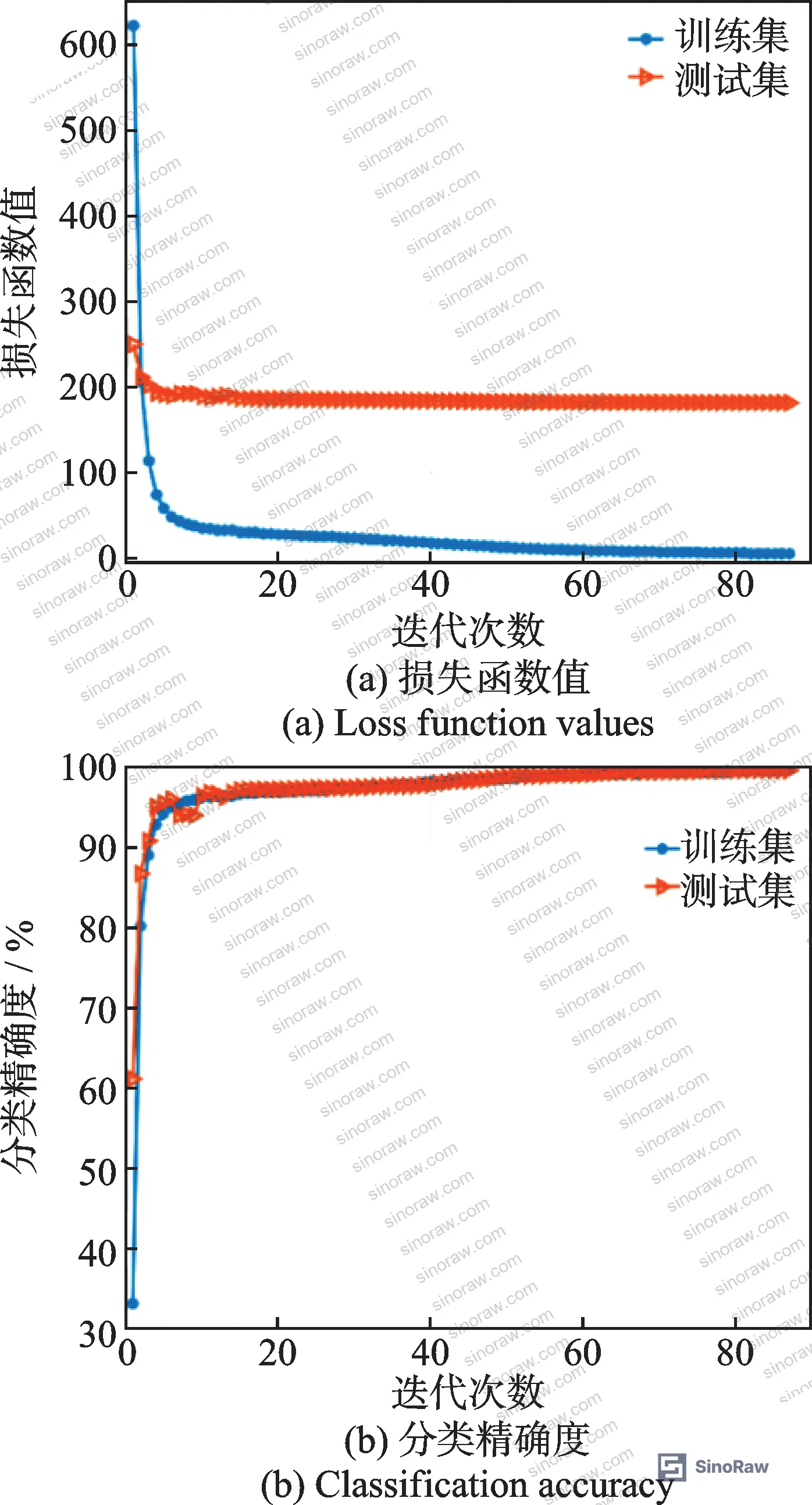
The training loss function converged to the interval [181.6, 181.7] for the test set after 60 epochs, with training and test accuracy tracking closely — confirming that the model generalized well and was not overfit to training data. Ten repeated trials confirmed the stability advantage of CNN-BOA, with standard deviation far below any of the comparison models.
Industry observation: field deployments of AE-based condition monitoring have historically been limited by two factors — sensor placement sensitivity and model brittleness under operating condition changes. The dual-channel AE sensor arrangement used in this work, with both sensors mounted at 45° on the radial plane of the seal cover as close as physically possible to the test seal ring, is a placement protocol that reduces signal attenuation artifacts. Very few commercially available seal monitoring packages specify sensor mounting angle and proximity constraints in their installation documentation. If a supplier’s installation guide does not address this, ask why.
For monitoring systems intended for environments subject to environmental compliance review, verify that the equipment also carries ISO 14001:2015 Environmental management systems certification from the manufacturing facility — particularly relevant for systems destined for chemical processing or energy sector installations where environmental audit requirements apply.
Practical Guidance for Buyers #
When specifying AE-based condition monitoring for non-contact rotary seal applications, the test data from this research gives you concrete numbers to work with rather than vendor claims.
The minimum viable AE acquisition system for multi-fault seal diagnostics should support a sampling rate of at least 1.25 MHz and a sensor bandwidth spanning 13 to 1035 kHz. Below these thresholds, you will not reliably capture the signal content that distinguishes spring degradation from end-face wear. The 14,000-sample validated dataset generated here represents a meaningful benchmark — ask any supplier offering a seal monitoring solution how large their training dataset is and under what pressure and speed conditions it was collected.
The confusion matrix data tells you something actionable: SF and PF states are the hardest to separate. If your application involves spring-loaded non-contact seals in a condition where partial spring failure is a known degradation pathway, verify that the supplier’s model has been specifically validated on these two states. A supplier who cannot produce per-class precision data for SF and PF is either using an underperforming model or has not tested it rigorously enough.
Our sourcing team at sinoraw.com works with Guangzhou-based procurement specialists who regularly connect overseas engineers with qualified Chinese manufacturers of industrial sensing systems, MRO components, and condition monitoring equipment — if you are evaluating AE sensor suppliers or diagnostic platform vendors for seal monitoring applications, we can help you structure your RFQ and verify supplier technical competence before you commit. Need help identifying qualified suppliers for non-contact seal monitoring systems? Talk to our sourcing team →
Supplier Qualification Questions #
- What is the AE signal acquisition bandwidth of your sensor system, and can you confirm it covers the 13 to 1035 kHz range required for distinguishing dry friction from mixed lubrication states in non-contact rotary seals?
- Can you provide a confusion matrix showing per-class classification precision for at least six fault conditions including spring failure and partial spring failure, with both states present simultaneously in the test dataset?
- What is the validated mean classification accuracy of your diagnostic model across all supported fault categories, and was this measured over 10 repeated independent trials to confirm standard deviation stability?
- What hyperparameter optimization method was used to train your classification model — manual tuning, random search, or an automated approach such as Bayesian optimization — and can you show the optimization convergence history?
- At what motor speed and line pressure were your training and validation datasets collected, and do you have data specifically covering the startup/shutdown speed range of 50 to 600 r/min where mixed lubrication transitions occur?
Sourcing Checklist #
- ☐ AE acquisition system supports sampling rate ≥1.25 MHz and sensor bandwidth 13–1035 kHz
- ☐ Supplier provides confusion matrix data covering all 7 fault states including spring failure (SF) and partial spring failure (PF) as separate classes
- ☐ Model mean classification accuracy ≥99% across 7 operational states, validated over ≥10 repeated trials
- ☐ Standard deviation of classification accuracy across repeated trials is lower than comparison random-search baseline (CNN-RR equivalent: 99.3760%)
- ☐ Training dataset contains ≥2,000 samples per fault class collected under controlled pressure (0.1 MPa) and defined speed conditions
- ☐ Dual-channel AE sensor mounting protocol specified, including angular placement (45°) and proximity to seal ring
- ☐ Supplier holds ISO 9001:2015 certification; facility environmental compliance verifiable under ISO 14001:2015
Key Specifications Table #
| Parameter | Recommended Value | Verification Method |
|---|---|---|
| AE sampling rate | ≥1.25 MHz (system max 2.5 MHz) | Acquisition system datasheet verification |
| AE sensor frequency bandwidth | 13–1035 kHz | Calibration certificate, frequency response curve |
| Model classification accuracy (7-class) | ≥99.7% mean across 10 repeated trials | Confusion matrix + repeated trial standard deviation report |
| Training dataset size (per class) | ≥2,000 samples per fault category (14,000 total for 7 classes) | Dataset documentation with sampling conditions |
| Test/train split ratio | 30% test / 70% training, no overlap | Cross-validation protocol documentation |
| Operating pressure during validation | 0.1 MPa | Test rig certification or calibration record |
| Motor speed range covered | 50–1000 r/min (including startup: 50 and 600 r/min) | Test log with speed controller data |
Can’t find a supplier meeting these specs? Submit your requirements and we’ll match you within 48 hours.
References #
Data source: Acoustic Emission Signal-Based Fault Diagnosis and Condition Identification of Non-Contact Rotary Mechanical Seals Using Bayesian-Optimized Convolutional Neural Networks, J.-R. Deng et al., Mechanical Systems and Signal Processing, 2025
Frequently Asked Questions #
What is the difference between dry friction, mixed lubrication, and fluid dynamic lubrication in a non-contact rotary seal?
These three states represent the tribological spectrum the seal experiences depending on rotational speed. At low speeds (startup/shutdown), the spiral groove cannot generate sufficient dynamic pressure to maintain a full gas film, resulting in dry friction — direct face contact with the highest wear risk. At intermediate speeds, partial gas film support occurs (mixed lubrication). At design operating speed, the spiral groove pumps gas inward and generates a film of only a few micrometers that carries the full face-closing force — this is fluid dynamic lubrication, the intended operating state with minimal friction and leakage.
Why can acoustic emission signals distinguish these states when pressure and temperature monitoring cannot?
Pressure and temperature are bulk parameters that change slowly and only reflect serious degradation after the fact. AE signals are generated at microsecond timescales by the actual contact mechanics at the seal face — asperity collisions, micro-fracture events, and gas film fluctuations each produce distinct high-frequency signatures in the 13–1035 kHz range. This makes AE fundamentally more sensitive to early-stage fault development than conventional monitoring parameters.
Why are spring failure and partial spring failure the hardest fault states to classify separately?
Because partial spring failure is a degradation intermediate of full spring failure — the time-frequency signatures of both states share significant spectral overlap. Even after deep convolutional feature extraction, 7 SF samples were misclassified as PF and 5 PF samples as SF in the study dataset. This is the honest limitation of current AE-based seal diagnostics and should be factored into any monitoring system specification where spring degradation is the primary failure mechanism of concern.
Is a 64×64 pixel time-frequency image sufficient resolution for reliable fault classification?
For the seven-class problem studied here, yes — the CNN-BOA model achieved 99.7023% accuracy with 64×64 CWT images as input. Higher resolution inputs would increase computational cost without a demonstrated accuracy benefit for this specific fault set. The resolution adequacy is confirmed by the t-SNE visualization showing clean inter-class separation after the fully connected layers.
What minimum dataset size should I require from a supplier offering a trained seal diagnostic model?
Based on the experimental benchmark, 2,000 samples per fault class is the validated threshold — giving 14,000 total samples for a 7-class problem. A supplier whose model was trained on fewer than 1,000 samples per class should be asked to justify their generalization claims, particularly for the SF/PF pair which shows the most overlap and requires the largest sample count to resolve reliably.
Published by sinoraw.com Technical Team | Request a sourcing quote


